\[\newcommand{\N}{\mathbb N}
\newcommand{\Z}{\mathbb Z}
\newcommand{\Q}{\mathbb Q}
\newcommand{\R}{\mathbb R}
\newcommand{\C}{\mathbb C}
\newcommand{\ba}{\mathbf{a}}
\newcommand{\bb}{\mathbf{b}}
\newcommand{\bc}{\mathbf{c}}
\newcommand{\bd}{\mathbf{d}}
\newcommand{\be}{\mathbf{e}}
\newcommand{\bff}{\mathbf{f}}
\newcommand{\bh}{\mathbf{h}}
\newcommand{\bi}{\mathbf{i}}
\newcommand{\bj}{\mathbf{j}}
\newcommand{\bk}{\mathbf{k}}
\newcommand{\bN}{\mathbf{N}}
\newcommand{\bn}{\mathbf{n}}
\newcommand{\bo}{\mathbf{0}}
\newcommand{\bp}{\mathbf{p}}
\newcommand{\bq}{\mathbf{q}}
\newcommand{\br}{\mathbf{r}}
\newcommand{\bs}{\mathbf{s}}
\newcommand{\bT}{\mathbf{T}}
\newcommand{\bu}{\mathbf{u}}
\newcommand{\bv}{\mathbf{v}}
\newcommand{\bw}{\mathbf{w}}
\newcommand{\bx}{\mathbf{x}}
\newcommand{\by}{\mathbf{y}}
\newcommand{\bz}{\mathbf{z}}
\newcommand{\bzero}{\mathbf{0}}
\newcommand{\nv}{\mathbf{0}}
\newcommand{\cA}{\mathcal{A}}
\newcommand{\cB}{\mathcal{B}}
\newcommand{\cC}{\mathcal{C}}
\newcommand{\cD}{\mathcal{D}}
\newcommand{\cE}{\mathcal{E}}
\newcommand{\cF}{\mathcal{F}}
\newcommand{\cG}{\mathcal{G}}
\newcommand{\cH}{\mathcal{H}}
\newcommand{\cI}{\mathcal{I}}
\newcommand{\cJ}{\mathcal{J}}
\newcommand{\cK}{\mathcal{K}}
\newcommand{\cL}{\mathcal{L}}
\newcommand{\cM}{\mathcal{M}}
\newcommand{\cN}{\mathcal{N}}
\newcommand{\cO}{\mathcal{O}}
\newcommand{\cP}{\mathcal{P}}
\newcommand{\cQ}{\mathcal{Q}}
\newcommand{\cR}{\mathcal{R}}
\newcommand{\cS}{\mathcal{S}}
\newcommand{\cT}{\mathcal{T}}
\newcommand{\cU}{\mathcal{U}}
\newcommand{\cV}{\mathcal{V}}
\newcommand{\cW}{\mathcal{W}}
\newcommand{\cX}{\mathcal{X}}
\newcommand{\cY}{\mathcal{Y}}
\newcommand{\cZ}{\mathcal{Z}}
\newcommand{\rA}{\mathrm{A}}
\newcommand{\rB}{\mathrm{B}}
\newcommand{\rC}{\mathrm{C}}
\newcommand{\rD}{\mathrm{D}}
\newcommand{\rE}{\mathrm{E}}
\newcommand{\rF}{\mathrm{F}}
\newcommand{\rG}{\mathrm{G}}
\newcommand{\rH}{\mathrm{H}}
\newcommand{\rI}{\mathrm{I}}
\newcommand{\rJ}{\mathrm{J}}
\newcommand{\rK}{\mathrm{K}}
\newcommand{\rL}{\mathrm{L}}
\newcommand{\rM}{\mathrm{M}}
\newcommand{\rN}{\mathrm{N}}
\newcommand{\rO}{\mathrm{O}}
\newcommand{\rP}{\mathrm{P}}
\newcommand{\rQ}{\mathrm{Q}}
\newcommand{\rR}{\mathrm{R}}
\newcommand{\rS}{\mathrm{S}}
\newcommand{\rT}{\mathrm{T}}
\newcommand{\rU}{\mathrm{U}}
\newcommand{\rV}{\mathrm{V}}
\newcommand{\rW}{\mathrm{W}}
\newcommand{\rX}{\mathrm{X}}
\newcommand{\rY}{\mathrm{Y}}
\newcommand{\rZ}{\mathrm{Z}}
\newcommand{\pv}{\overline}
\newcommand{\iu}{\mathrm{i}}
\newcommand{\ju}{\mathrm{j}}
\newcommand{\im}{\mathrm{i}}
\newcommand{\e}{\mathrm{e}}
\newcommand{\real}{\operatorname{Re}}
\newcommand{\imag}{\operatorname{Im}}
\newcommand{\Arg}{\operatorname{Arg}}
\newcommand{\Ln}{\operatorname{Ln}}
\DeclareMathOperator*{\res}{res}
\newcommand{\re}{\operatorname{Re}}
\newcommand{\im}{\operatorname{Im}}
\newcommand{\arsinh}{\operatorname{ar\,sinh}}
\newcommand{\arcosh}{\operatorname{ar\,cosh}}
\newcommand{\artanh}{\operatorname{ar\,tanh}}
\newcommand{\sgn}{\operatorname{sgn}}
\newcommand{\diag}{\operatorname{diag}}
\newcommand{\proj}{\operatorname{proj}}
\newcommand{\rref}{\operatorname{rref}}
\newcommand{\rank}{\operatorname{rank}}
\newcommand{\Span}{\operatorname{span}}
\newcommand{\vir}{\operatorname{span}}
\renewcommand{\dim}{\operatorname{dim}}
\newcommand{\alg}{\operatorname{alg}}
\newcommand{\geom}{\operatorname{geom}}
\newcommand{\id}{\operatorname{id}}
\newcommand{\norm}[1]{\lVert #1 \rVert}
\newcommand{\tp}[1]{#1^{\top}}
\renewcommand{\d}{\mathrm{d}}
\newcommand{\sij}[2]{\bigg/_{\mspace{-15mu}#1}^{\,#2}}
\newcommand{\abs}[1]{\lvert#1\rvert}
\newcommand{\pysty}[1]{\left[\begin{array}{@{}r@{}}#1\end{array}\right]}
\newcommand{\piste}{\cdot}
\newcommand{\qedhere}{}
\newcommand{\taumatrix}[1]{\left[\!\!#1\!\!\right]}
\newenvironment{augmatrix}[1]{\left[\begin{array}{#1}}{\end{array}\right]}
\newenvironment{vaugmatrix}[1]{\left|\begin{array}{#1}}{\end{array}\right|}
\newcommand{\trans}{\mathrm{T}}
\newcommand{\EUR}{\text{\unicode{0x20AC}}}
\newcommand{\SI}[3][]{#2\,\mathrm{#3}}
\newcommand{\si}[2][]{\mathrm{#2}}
\newcommand{\num}[2][]{#2}
\newcommand{\ang}[2][]{#2^{\circ}}
\newcommand{\meter}{m}
\newcommand{\metre}{\meter}
\newcommand{\kilo}{k}
\newcommand{\kilogram}{kg}
\newcommand{\gram}{g}
\newcommand{\squared}{^2}
\newcommand{\cubed}{^3}
\newcommand{\minute}{min}
\newcommand{\hour}{h}
\newcommand{\second}{s}
\newcommand{\degreeCelsius}{^{\circ}C}
\newcommand{\per}{/}
\newcommand{\centi}{c}
\newcommand{\milli}{m}
\newcommand{\deci}{d}
\newcommand{\percent}{\%}
\newcommand{\Var}{\operatorname{Var}}
\newcommand{\Cov}{\operatorname{Cov}}
\newcommand{\Corr}{\operatorname{Corr}}
\newcommand{\Tasd}{\operatorname{Tasd}}
\newcommand{\Ber}{\operatorname{Ber}}
\newcommand{\Bin}{\operatorname{Bin}}
\newcommand{\Geom}{\operatorname{Geom}}
\newcommand{\Poi}{\operatorname{Poi}}
\newcommand{\Hyperg}{\operatorname{Hyperg}}
\newcommand{\Tas}{\operatorname{Tas}}
\newcommand{\Exp}{\operatorname{Exp}}
\newcommand{\tdist}{\operatorname{t}}
\newcommand{\rd}{\mathrm{d}}
\newcommand{\oiint}{\unicode{x222F}}\]
Muuttujanvaihto tasointegraalissa
Pintaintegraalin erikoistapauksena saadaan tasointegraalin muuttujanvaihdon kaava,
joka saattaa olla ennestään tuttu aikaisemmilta kursseilta.
Tarkastellaan siis muuttujanvaihtoa (change of variables)
\[\begin{split}\begin{cases}
x=x(u,v) &\\
y=y(u,v) & \\
\end{cases}\end{split}\]
tasoalueelta \(\Omega\subset \mathbf{R}^2\) alueelle \(D\subset \mathbf{R}^2\). Oletetaan, että muunnos
on bijektiivinen (eli pisteet \((u,v)\in \Omega\) vastaavat yksikäsitteisellä tavalla pisteitä \((x,y)\in D\)),
mahdollisesti alueiden reunoja lukuun ottamatta, ja jatkuvasti derivoituva alueen
\(\Omega\) sisällä. Lisäksi täytyy olettaa, että alueiden reunat ovat paloittain
sileitä käyriä. Kirjoittamalla
\[\mathbf{r}(u,v) = (x(u,v),y(u,v),0)\]
muuttujanvaihto voidaan tulkita pinnan \(D\times \{ 0\}\subset \mathbf{R}^3\) parametrisoinniksi,
jossa normaalivektori on muotoa
\[\begin{split}\mathbf{N} = \mathbf{r}_u\times \mathbf{r}_v
=\left|
\begin{matrix}
\mathbf{i} & \mathbf{j} &\mathbf{k} \\
x_u & y_u & 0\\
x_v & y_v & 0\\
\end{matrix}
\right|
=\left| \begin{matrix}
x_u & y_u \\
x_v & y_v\\
\end{matrix}
\right| \mathbf{k}.\end{split}\]
Pinta-alan suurennussuhteeksi saadaan
\[\begin{split}\|\mathbf{N}\| =
\operatorname{abs}\left| \begin{matrix}
x_u & y_u \\
x_v & y_v\\
\end{matrix}\right|
=\left| \frac{\partial (x,y)}{\partial (u,v)}\right|,\end{split}\]
jossa abs tarkoittaa determinantin itseisarvoa ja viimeinen lauseke on
(ennestään tuttu?) kaksiulotteisen muuttujanvaihdon Jacobin determinantin (Jacobian determinant)
lyhennysmerkintä.
Näin saadaan seuraava tulos.
Lause 5.6.1
Tarkastellaan yllä esitettyä tasoalueiden välistä muuttujanvaihtoa \(\Omega \to D\).
Jos \(f\colon D\to \R\) on (paloittain) jatkuva funktio, niin
\[\iint_D f\, dA = \iint_{\Omega} f(x(u,v),y(u,v))\left| \frac{\partial (x,y)}{\partial (u,v)}\right| \, du\, dv.\]
Huomautus 5.6.2
Jacobin determinantista täytyy siis ottaa itseisarvo, sillä muuten positiivisen
funktion tasointegraalista voi tulla negatiivinen. Esimerkiksi peilauksessa \((x,y)\mapsto (x,-y)\)
kaikkien joukkojen pinta-alat pysyvät samoina (tapaus \(f=1\) = vakio), mutta muunnoksen
Jacobin determinantti on \(-1\).
Ehdottomasti tärkein tapaus on integrointi napakoordinaatistossa, jossa \(x=r\cos\theta\), \(y=r\sin\theta\),
ja pinta-alan suurennusuhteeksi saadaan \(r\). Tämä seuraa erikoistapauksena seuraavasta esimerkistä,
mutta se on johdettu geometrisella tarkastelulla jo esimerkissä 4.1.4.
Esimerkki 5.6.3
Ellipsin
\[\frac{x^2}{a^2}+\frac{y^2}{b^2} = 1\]
rajaaman tasoalueen
\[\frac{x^2}{a^2}+\frac{y^2}{b^2} \le 1\]
parametrisointi saadaan venyttämällä napakoordinaatteja puoliakseleiden
pituuksilla \(a\) ja \(b\):
\[\begin{split}\begin{cases}
x=ar\cos\theta &\\
y=br\sin \theta, &\\
\end{cases}\end{split}\]
kun \(0\le r\le 1\) ja \(0\le \theta \le 2\pi\). Pinta-alan suurennussuhteeksi saadaan
\[\begin{split}\frac{\partial (x,y)}{\partial (r,\theta)}
=\left| \begin{matrix}
x_r & y_r \\
x_{\theta} & y_{\theta}\\
\end{matrix}
\right|
=\left| \begin{matrix}
a\cos \theta & b\sin\theta \\
-ar\sin\theta & br\cos\theta\\
\end{matrix}\right|
=abr.\end{split}\]
Ellipsin pinta-ala on
\[A= \int_0^{2\pi}\int_0^1 abr\, dr\, d\theta = \pi ab.\]
Erikoistapauksessa \(a=b=R\) saadaan \(R\)-säteisen ympyrän pinta-ala \(\pi R^2\).
Ellipsin pinta-ala voidaan päätellä myös alkeellisesti, koska ellipsi saadaan yksikköympyrästä (pinta-ala = \(\pi\))
venyttämällä \(x\)-suunnassa kertoimella \(a\) ja \(y\)-suunnassa kertoimella \(b\), jolloin pinta-ala
skaalautuu (venytyssuuntien kohtisuuruuden vuoksi) kertoimella \(ab\).
Esimerkki 5.6.4
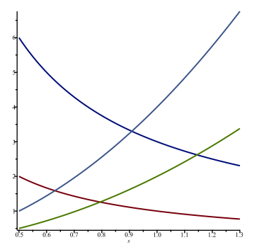
Laske käyrien \(xy=1\), \(xy=3\), \(y=2x^2\) ja \(y=4x^2\) rajaaman alueen \(D\) pinta-ala.
Piilota/näytä ratkaisu
Valitaan uusiksi muuttujiksi \(u=xy\) ja \(v=y/x^2\), koska tällöin käyrien
rajaamaa aluetta kuvaavat yksinkertaiset ehdot \(1\le u\le 3\) ja \(2\le v\le 4\),
ts. parametrialue \(\Omega\) on neliö!
Muunnoksen Jacobin determinantti voidaan laskea kahdella tavalla: suoraviivainen, mutta hankala,
tai helpompi ovela tapa. Hankalassa tavassa ratkaistaan ensin (esimerkiksi jakamalla yhtälöt puolittain)
\(x=(u/v)^{1/3}\) ja \(y=(u^2v)^{1/3}\). Tämän jälkeen voidaan laskea Jacobin determinantti
\(\frac{\partial (x,y)}{\partial (u,v)}\) määritelmän kaavalla. Helpomassa laskutavassa lasketaan
ensin käänteismuunnoksen determinantti
\[\begin{split}\frac{\partial (u,v)}{\partial (x,y)} =
\left| \begin{matrix}
u_x & v_x \\
u_y & v_y\\
\end{matrix}\right|
=
\left| \begin{matrix}
y & -2y/x^3 \\
x & 1/x^2\\
\end{matrix}\right| = \frac{3y}{x^2} =3v.\end{split}\]
Muunnoksen ja käänteismuunnoksen suurennussuhteet ovat toistensa käänteislukuja (mieti miksi!),
joten
\[\frac{\partial (x,y)}{\partial (u,v)} = \frac{1}{3v}.\]
Tämän avulla pinta-alaksi saadaan
\[A=\iint_D 1 \, dA = \int_1^3\int_2^4\frac{dv}{3v}\, du = \frac{1}{3}(3-1)(\ln 4-\ln 2) = \frac{2}{3}\ln 2.\]